
Thermomechanics
Coupling from Mechanical Field to Thermal Field
The heat generated by the mechanical field serves as the major coupling from the mechanical field to the thermal field. The governing equation of the thermal field, i.e., heat equation, is first recalled to mathematically formulate this coupling: \[\frac{\partial \left(\rho CT\right)}{\partial t} =\nabla \cdot \left(\lambda \nabla T\right)-\nabla \cdot \left(\rho CTv\right)+g, \] where $\rho $ is the density, $C$ is the gravimetric heat capacity, $T$ is temperature, $\lambda $ is the thermal conductivity, $v$ is the velocity of material particles, and $g$ is the heat source.
For both friction and plasticity deformation, the heat source can be related to the rate of the work done on the material point of interest: \[g=\eta \frac{dW}{dt} ,\] where $\eta $ is the ratio between the generated heat and the total mechanical energy input or energy dissipation, $W$. For plasticity, the above total mechanical energy dissipation in the plastic deformation can be formulated as \[W=-\sigma :\dot{\varepsilon }_{{\rm p}} , \] where $\dot{\varepsilon }_{{\rm p}} $ is the plastic strain rate. The heat source in the thermal field then becomes \[g=\eta \sigma :\dot{\varepsilon }_{{\rm p}} . \] The value of $\eta $ is usually low in friction. However, it could be much higher in the plastic deformation. For example, experiments with an alloy made of Ti, Al and Cu showed that $\eta $ could be as high as 70% during high strain rate plastic deformation [Hapoor and Nemat-Nasser, 1998]. In a liquid, it is common to assume that most of the energy dissipation goes to the internal energy of the liquid, especially the kinetic energy of the liquid molecules. Therefore, $\eta$ is approximately 1. The heat source attributed to the viscous energy dissipation in the fluid can be formulated as \[g=\sigma :\nabla \dot{u}, \] where $\dot{u}$ is the velocity vector. For compressible Newtonian fluids, a detailed formulation of the viscous dissipation is \[g=\mu \left[\begin{array}{l} {2\left(\frac{\partial u}{\partial x} \right)^{2} +2\left(\frac{\partial v}{\partial y} \right)^{2} +2\left(\frac{\partial w}{\partial z} \right)^{2} } \\ {+\left(\frac{\partial v}{\partial x} +\frac{\partial u}{\partial y} \right)^{2} +\left(\frac{\partial w}{\partial y} +\frac{\partial v}{\partial z} \right)^{2} +\left(\frac{\partial u}{\partial z} +\frac{\partial w}{\partial x} \right)^{2} } \end{array}\right]+\lambda \left(\nabla \cdot u\right)^{2} ,\] where $\mu $ and $\lambda $ are the viscosities associated with the shearing deformation and volume change, respectively; and $u$, $v$, and $w$ are the components of the flow velocity along three mutually-perpendicular directions in the Cartesian coordinate system.
$\space$Coupling from Thermal Field to Mechanical Field
In order to derive the governing equation, let get back to the equation of equilibrium, \[\nabla \cdot \sigma +f=0. \] The stress $\sigma $ in the above equation is the elastic stress. However, the strain obtained from the strain-displacement relationship is the total strain $\varepsilon $ instead of the elastic strain $\varepsilon _{{\rm e}} $. Therefore, the above equation with the thermal strain term can be rewritten considering $\sigma =D:\varepsilon _{{\rm e}} =D:\left(\varepsilon -\varepsilon _{{\rm T}} \right)$, \[\nabla \cdot \left[D:\left(\varepsilon -\varepsilon _{{\rm T}} \right)\right]+f=0. \] Substituting the formulation of the stiffness matrix for linear elasticity into the above equilibrium equation, we can obtain the following non-isothermal Navier's equation by following the derivation procedure used in the chapter for the mechanical field: \[\mu \nabla ^{2} u+\left(\mu +\lambda \right)\nabla \left(\nabla \cdot u\right)+f-3\alpha K\nabla \left[\left(T-T_{0} \right)I\right]=0, \] or equivalently, \[\nabla \cdot \left[D:\frac{1}{2} \left(\nabla u-\left(\nabla u\right)^{{\rm T}} \right)-3\alpha K\left(T-T_{0} \right)I\right]+f=0, \] where $D$ is the stiffness tensor (fourth-order tensor) and $I$ is \[I=\left[\begin{array}{ccc} {1} & {0} & {0} \\ {0} & {1} & {0} \\ {0} & {0} & {1} \end{array}\right]. \] Once the displacement is obtained by solving the above governing equation, the stress will need to be calculated with the following equation: \[\sigma =D:\frac{1}{2} \left(\nabla u-\left(\nabla u\right)^{{\rm T}} \right)-3\alpha K\left(T-T_{0} \right)I. \] Please note that the stress and displacement in the above equation are written using the tensor notation instead of the Voigt notation.
$\space$Example
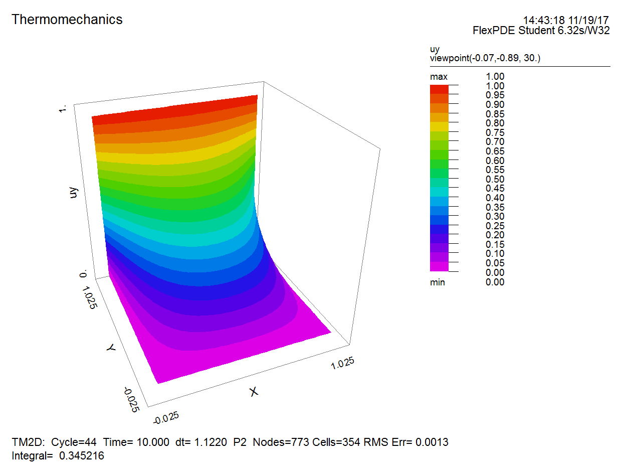
A 2D (plane-strain) square object with a side length of 1 m has an initial temperature of 273.15 K. The top boundary gets into contact with a water bath with a temperature of 293.15 K while all the other boundaries are connected to a water bath with a temperature of 273.15 K. The material of the object has a thermal diffusivity of $1\times 10^{-7} $${{\rm m}^{2}/{\rm s}}$. The two sides of the object are fixed while the top and bottom are constrained using rollers. The Young's modulus is 10 GPa and Poisson's ratio is 0.2. The linear thermal expansion coefficient of the material is $1\times 10^{-5}$ $1/{\rm K} $. Please compute $\sigma _{y} $ in the domain at $t=10$.
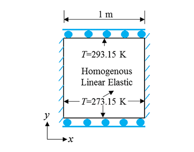
Results: