Multiphysics Learning & Networking

Introduction

Electrokinetics includes a family of phenomena resulting from the distributions of the charges and electrical potential at interfaces between two different phases. In porous materials, these two phases primarily refer to the solid phase such as clay particles and the liquid phase such as water. Such two dissimilar phases usually have different chemical potentials. Upon contact, it is very likely that one of the phases, like water, is a polar liquid and will tend to orient its (dipolar) molecules in a particular direction at the interface and consequently generate a potential difference. The existence of this special electric field gives rise to various electrokinetic phenomena.

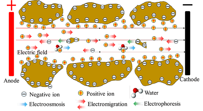
As shown in the following figure for soils, water moves as polarized water molecules are attached to cations, which are mobilized by an external electric field. Meanwhile, as the external electric field is also applied to the particles with excess charges, the suspended particles can be moved, leading to another significant electrokinetic phenomenon: electrophoresis. In addition, charged ions and ion complexes also migrate due to the electric field, resulting in the phenomenon of electromigration.

Governing Equations

Unlike electrophoresis, electroosmosis contributes to the mass transfer of the continuous phase instead of the dispersed phase. Accordingly, the water movement equation should be used. For a more general variably saturated porous material, an extension to Richards' equation [Richards 1931] for unsaturated water flow could be expressed as \[\phi \frac{\partial S_{w} }{\partial h} \frac{\partial h}{\partial t} +\nabla \cdot J_{{\rm m}} =0, \] where $S_{w} $ is the degree of saturation, $t$ is the time, $\phi $ is the porosity, $h$ is the hydraulic pressure head, and $J_{{\rm m}} $ is flux or the extended Darcy velocity. In this case, let us consider the water flow caused by both the water pressure/potential gradient and the electrical potential gradient, \[J_{{\rm m}} =J_{{\rm H}} +J_{{\rm EO}} =-K_{{\rm H,0}} K_{{\rm H}r} \nabla (h+z)-K_{{\rm EM,0}} K_{{\rm EM},r} \nabla \psi \] where $K_{{\rm H,0}} $ is the intrinsic (saturated) hydraulic conductivity (due to water head), $K_{{\rm H}r} $is the coefficient of relative hydraulic conductivity, $z$ is the coordinate along the gravity direction, $K_{{\rm EM,0}} $ is the intrinsic (saturated) electroosmotic conductivity, $K_{{\rm EM},r} $ is the coefficient of relative electroosmotic conductivity, and $\psi $ is the electric potential. From the above two equations, the governing equation for the coupled unsaturated water flow including electroosmosis turns into \[\phi \frac{\partial S_{w} }{\partial h} \frac{\partial h}{\partial t} =\nabla \cdot \left[K_{{\rm H,0}} K_{{\rm H}r} \nabla (h+z)+K_{{\rm EM,0}} K_{{\rm EM},r} \nabla \psi \right].\] According to Ohm's law, the electrical current density $J_{{\rm E}} $ can be expressed as [Ohm, 1827]: \[J_{{\rm E}} =-\sigma \nabla \psi , \] where $\sigma $ is the conductivity of the soil. Due to the conservation of electrical charges, the governing equation for the electrical potential could be obtained by placing a divergence operator on the two sides of the Ampere equation, leading to \[-\nabla \cdot J_{{\rm E}} =\varepsilon \frac{\partial \psi }{\partial t} , \] where $\varepsilon $ is the absolute permittivity of the soil, which is very small. Combining the above two equations, the governing equation for the electrostatics in soils could be obtained as follows \[\nabla \cdot (\sigma \nabla \psi )=\varepsilon \frac{\partial \psi }{\partial t} . \] In addition to the water movement and electrostatics, the conservation of ions is also usually of major interest in electrokinetics applications. The governing equation for ion transport can be obtained by extending the equation introduced in the chapter for the concentration field: \[\frac{\partial c}{\partial t} =\underbrace{-\nabla \cdot \left(-D_{{\rm diff}} \nabla c\right)}_{{\rm diffusion+\; dispersion}}-\underbrace{\nabla \cdot \left(J_{{\rm EM}} +J_{{\rm EP}} \right)}_{{\rm dispersion}}-\underbrace{\nabla \cdot \left(vc\right)}_{{\rm advection}}. \] All the flux and velocity terms in the above equation have been introduced in the previous sections.

Typical Auxiliary Equations

The degree of saturation could be expressed as a function of the hydraulic pressure head: \[S=\left[1+\left(-\alpha h\right)^{n} \right]^{-m} , \] where typical values for the fitting constants are $\alpha =8.51{\kern 1pt} {\kern 1pt} {\kern 1pt} {\kern 1pt} {\kern 1pt} {\rm m}^{-1} $, $n=1.31$, and $m=1-\frac{1}{n} $. It is also common to express the relative hydraulic conductivity as a function of the degree of saturation. Here we use a simple power rule: \[K_{{\rm H}r} ={\rm a}_{{\rm H}} \left(S\right)^{{\rm b}_{{}_{{\rm H}} } } , \] where typical values for the fitting constants are ${\rm a}_{{\rm H}} =1.0$ and $b_{{\rm H}} =5$. The electric conductivity of a soil has contributions from both the liquid and the solid phases: \[\sigma =\sigma _{{\rm l}} +\sigma _{{\rm s}} , \] where $\sigma _{{\rm l}} $ and $\sigma _{{\rm s}} $ are the electric conductivity components contributed by the liquid and the solid, respectively. $\sigma _{{\rm l}} $ is termed the bulk electric conductivity of the pore liquid in some literature. This quantity changes with both the degree of saturation, tortuosity, and the types and concentrations of the ions in the liquid. Theoretically, $\sigma _{{\rm l}} $ can be formulated based on the theory of electromigration: \[\sigma _{{\rm l}} =\sigma _{{\rm w}} \theta \tau _{{\rm EK}} =\mu _{q}^{{\rm eff}} c{\rm F}=\frac{D_{{\rm diff}} \cdot z\cdot {\rm F}}{{\rm R}T} \theta \tau _{{\rm EK}} c{\rm F}, \] where $\sigma _{{\rm w}} $ is the true electric conductivity of the pore water and $\mu _{q}^{{\rm eff}} c$ gives out the number of ions (in mol) passing through a unit area per unit time under a unit electric field. One more auxiliary relationship is still needed to enable numerical simulation of electrokinetics in porous materials for tortuosity. Mattson et al [2002] employed a simple relationship between the tortuosity and the water content as follows \[\tau _{{\rm EK}} =\frac{{\rm F}_{\lambda } \left(\theta -\theta _{{\rm r}} \right)^{n+1} }{\theta _{{\rm sat}} } .\] where $\theta $, $\theta _{{\rm r}} $, and $\theta _{{\rm sat}} $ are the water content, immobile water content, and saturated water content, respectively; and ${\rm F}_{\lambda } $ is a constant, i.e., 1.58.

Example

An experiment was conducted using a mixture of a play sand (poorly graded fine sand) and a clay (high plasticity) with a dry mass ratio of 1:1. The mixture was compacted gently using a miniature compactor and the final specific gravity is 1.9. The compacted soil sample sat for 24 hours to allow for the water content to become uniform and the sample was also covered with a plastic sheet to reduce the effects of evaporation.

Electrodes made of copper robs were placed on two sides of the plastic tank to trigger the electrokinetic process. A voltage of 20 Volts was placed on the two electrodes: 10 V and -10 V on the two electrodes. The tank had (inner) dimensions of 37 cm (length) by 21 cm (width) by 22.5 cm (height). The electrodes extend to the bottom of the soil layer (also tank), which filled slightly over one half of the tank height to generate an approximately 1D problem.

Three water content sensors (Decagon GS3), connected to a data logger (Decagon EM50), were placed along the x-axis of the tank, whose positions are displayed in the following figure.

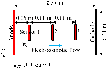
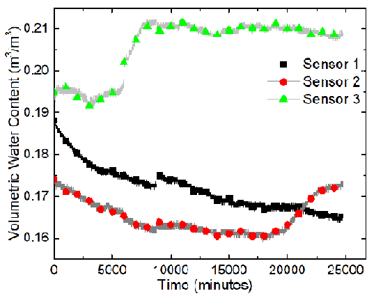
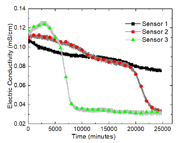
The sensors, from the left to the right, are named Sensor 1, Sensor 2, and Sensor 3. A program called ECH20 Utility was used to record the volumetric moisture content and the electric conductivity automatically. The GS3 water content sensors measure the variation of the electric conductivity between two of its probes. The program took measurements every minute. Data were recorded for about 417 hours. Temperatures of the soil sample were recorded using Type-K thermocouples and the built-in temperature sensors in the water content sensor.

The saturated hydraulic conductivity and saturated electroosmotic hydraulic conductivity are 5$\mathrm{\times}$10${}^{-8\ }$m/s and 1.5$\mathrm{\times}$10${}^{-9}$ m/s, respectively. The soil water characteristic curve, relative hydraulic conductivity, and relative electroosmotic conductivity are formulated with the given default values. The tortuosity is also calculated. The initial soil water pressure head is -0.08 m. The saturated and residual water contents are assumed to be 0.40 and 0 respectively. The concentrations of cations and anions in the pore water are both 8 mol/m${}^{3}$. The average diffusivity of cations and anions are 0.5$\mathrm{\times}$10${}^{-9}$ m${}^{2}$/s and 1.5$\mathrm{\times}$10${}^{-9}$ m${}^{2}$/s. The average valence is assumed to be 1 for both the cations and anions. The electric conductivity can be calculated using $\sigma _{{\rm s}} $=0.0032 S/m.

The results of the sand-clay mixture electrokinetics experiment are shown in terms of variations of the volumetric water content and electric conductivity at Sensors 1, 2, and 3 in the following two figures.