
Thermohydromechanics
Introduction
In porous materials, thermohydromechanics is one of the most common types of multiphysical phenomena in addition to the static poroelasticity. Thermohydromechanics is responsible for many applications related to unsaturated porous materials such as hydro-diffusion and subsidence, drying/hydration and shrinkage, frost heave, spalling, geothermal applications, and hydraulic cracking. We will show the establishment of the model using a bottom-up approach in contrast to the top-down approach using in static poroelasticity.
$\space$Thermal Field
To precisely formulate the energy transport in porous materials, a modified Fourier's equation with both conduction and convection terms can be adopted:
\[C_{{\rm a}} \frac{\partial T}{\partial t} +C_{{\rm w}} \nabla \left(JT\right)=\nabla \cdot \left(\lambda \nabla T\right),\]where $C_{{\rm w}} $ is the heat capacity of unfrozen water, $C_{{\rm a}} $ is the apparent heat capacity, $\lambda $ is the thermal conductivity, $T$ is the temperature, $t$ is time, and $J$ is the water flux from the hydraulic field. Both $C_{{\rm a}} $ and $\lambda $ are coupling variables. The moisture migration changes the soil composition and consequently $C_{{\rm a}} $ and $\lambda $, which in turn affects the heat transfer process. Multiple simple mathematical formulations are available for $C_{{\rm a}} $ and $\lambda $.
$\space$Hydraulic Field
For variably unsaturated porous materials, the fluid movement is generally described by the mixed-type Richards' equation, which has been proven to perform well in ensuring mass conservation. To extend the Richards' equation to allow for freezing/thawing, a term related to ice formation needs to be added to the left-hand side of the Richards' equation to obtain
\[\frac{\partial \theta _{{\rm w}} }{\partial t} +\frac{\rho _{{\rm i}} }{\rho _{{\rm w}} } \frac{\partial \theta _{{\rm i}} }{\partial t} =\nabla \cdot \left(\kappa _{{\rm Lh}} \nabla h+\kappa _{{\rm Lh}} i+\kappa _{{\rm LT}} \nabla T\right), \]where $\theta _{{\rm w}} $ is the volumetric content of water, $\theta _{{\rm i}} $ is the volumetric content of ice, $\rho _{{\rm w}} $ is the density of water, $\rho _{{\rm i}} $ is the density of ice, $\kappa _{{\rm Lh}} $ is the hydraulic conductivity, $\kappa _{{\rm LT}} $ is the hydraulic conductivity due to a thermal gradient, $i$ is the unit vector along the direction of gravity, and $h$ is the matric potential head (or pressure head). The matric potential head is the equivalent water head (unit: m) of the matric potential (negative water suction, unit: Pa). It is common to formulate the above equation in terms of the matric potential head, matric potential, total soil potential head, or total soil potential. But attention is needed to make sure the units of other terms are consistent with that of the selected dependent variable.
The hydraulic conductivity can be estimated by integrating the SWCC [Childs and Colis-George, 1950; Mualem, 1986; Fredlund et al., 1994). Most THM studies employed either the simplified van Genuchten's equation [van Genuchten, 1980, Hansson, 2004] or Fredlund and Xing's equation [Fredlund and Xing, 1994] to mathematically describe the SWCC. Corresponding approaches are then adopted to predict the hydraulic conductivity with the SWCC. Taking van Genuchten's equation for example, we have the following equation for the SWCC:
\[S_{{\rm e}} =\frac{\theta -\theta _{{\rm r}} }{\theta _{{\rm s}} -\theta _{{\rm r}} } =\left(1+\left|\alpha h\right|^{{\rm n}} \right)^{{\rm -m}} , \]where $S_{{\rm e}} $ is the effective saturation, $\theta _{{\rm s}} $ and $\theta _{{\rm r}} $ are the saturated and residual water content respectively, and $\alpha $,${\rm m}$, and${\rm n}$ are empirical parameters.
$\kappa _{{\rm Lh}} $ and $\kappa _{{\rm LT}} $ are hydraulic conductivities related to the pore water head and temperature, respectively. One set of widely accepted relationships for these parameters is
\[\kappa _{{\rm Lh}} =\kappa _{{\rm s}} S_{{\rm e}} \left[1-\left(1-S_{{\rm e}} {}^{\frac{{\rm 1}}{{\rm m}} } \right)^{{\rm m}} \right]^{2} ,\] \[\kappa _{{\rm LT}} =\kappa _{{\rm Lh}} \left(hG_{{\rm wT}} \frac{1}{\gamma _{0} } \frac{d\gamma }{dT} \right),\]where $\gamma $ denotes the surface tension of soil water, which is temperature-dependent and can be approximated using the following equation:
\[\gamma =75.6-0.1425T-2.38\times 10^{-4} T^{2} ,\]where $\gamma _{0} $ is the value of $\gamma $ at 25 ${}^{\circ } {\rm C}$ , i.e.,$\gamma _{0} =71.89\times 10^{-3} {\rm \; kg}\cdot {\rm m}^{{\rm 3}} $. The thermal induced hydraulic conductivity $\kappa _{{\rm LT}} $ is developed from thermodynamics [Philip and de Vries, 1957]. $G_{{\rm wT}} $ is a gain factor, which has a value around 7 for coarse-grained soils [Noborio et al., 1996].
When phase changes are involved, the generalized Clapeyron equation needs to be employed to describe the thermodynamic condition for the co-existence of water and ice. The local freezing point of the pore fluid can be obtained from the generalized Clapeyron equation:
\[\frac{dh}{dT} =\frac{L_{{\rm f}} }{{\rm g}T} ,\]where $h$ is the water head, $L_{{\rm f}} $is the latent heat of water, and ${\rm g}$ is gravitational acceleration.
$\space$Mechanical Field
The governing equation for the mechanical field is the Navier's equation, which incorporates the equation of motion, strain-displacement correlation, and the constitutive relationship. The equation equilibrium is introduced in a general tensor format as
\[\nabla \cdot \sigma +F=0,\]where $u$ is the displacement vector and $F$ is the body force vector.
The strain-displacement equation is
\[\varepsilon =\frac{1}{2} \left[\nabla u+\left(\nabla u\right)^{T} \right].\]The constitutive equation is
\[\sigma =C:\varepsilon ,\]where $\sigma $ is the Cauchy stress tensor, $C$ is the fourth-order tensor of material stiffness, $\varepsilon $ is the infinitesimal strain tensor, and the symbol ":" stands for double contraction.
In order to consider the influence of the thermal field and the hydraulic field on the mechanical field, the constitutive relationship for porous materials is formulated as
\[\sigma =D\varepsilon _{{\rm el}} +\sigma _{0} , \]where $D$ is the stiffness matrix of soil skeleton, $\sigma _{0} $ is the initial stress vector, and $\varepsilon _{{\rm el}} $ is the elastic strain which can be obtained from the following relationship,
\[\varepsilon =\varepsilon _{{\rm el}} +\varepsilon _{{\rm th}} +\varepsilon _{{\rm tr}} +\varepsilon _{{\rm hp}} +\varepsilon _{0} ,\]where $\varepsilon _{{\rm th}} $ is the strain caused by thermal expansion, e.g.,$\left[{\rm \alpha }(T-T_{{\rm ref}} ),{\rm \alpha }(T-T_{{\rm ref}} ),0\right]^{{\rm T}} $ in 2D; $\varepsilon _{{\rm tr}} $ is the strain caused by the phase change of water, which was approximated as $\left[0.09Q,0.09Q,0\right]^{{\rm T}} $ when a unit localization tensor in mixture theory is followed, where $Q$ is the degree of water phase transition, 0.09 is the relative change of volume when water turns into ice; $\varepsilon _{0} $ is the initial strain; and $\varepsilon _{{\rm hp}} $ is the strain resulting from the change in the matric potential, which is calculated using $\left[h/H,h/H,0\right]^{{\rm T}} $. $H$ is the poroelastic expansion coefficient in unsaturated soils. The value of H can be obtained through experimental measurement.
$\space$Example
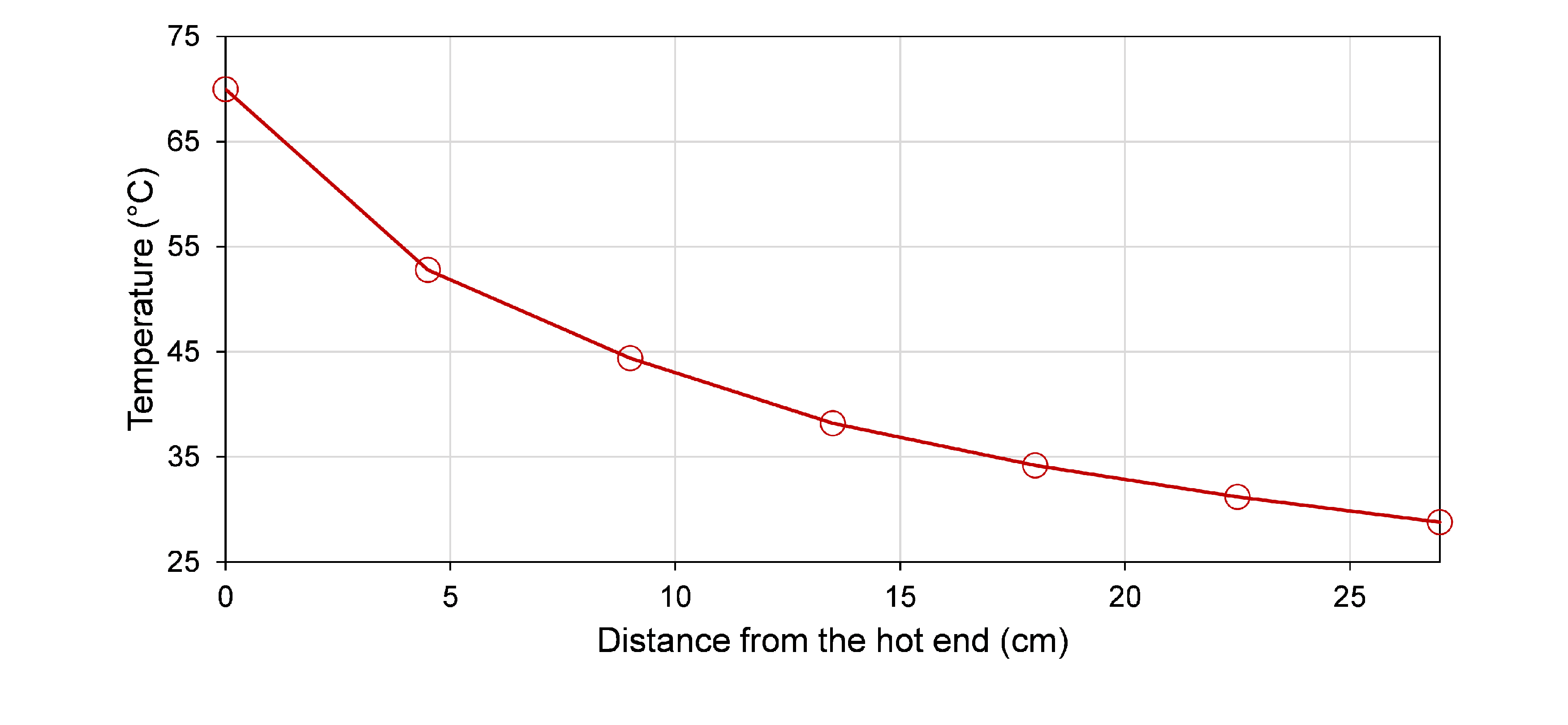
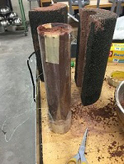
A cylindrical soil sample with a diameter of 0.06 m and a height of 0.26 m wrapped by thermal and hydraulic insulation materials on its side. The top and bottom are connected to solid objects at temperatures of 293.15 K and 343.15 K, respectively.
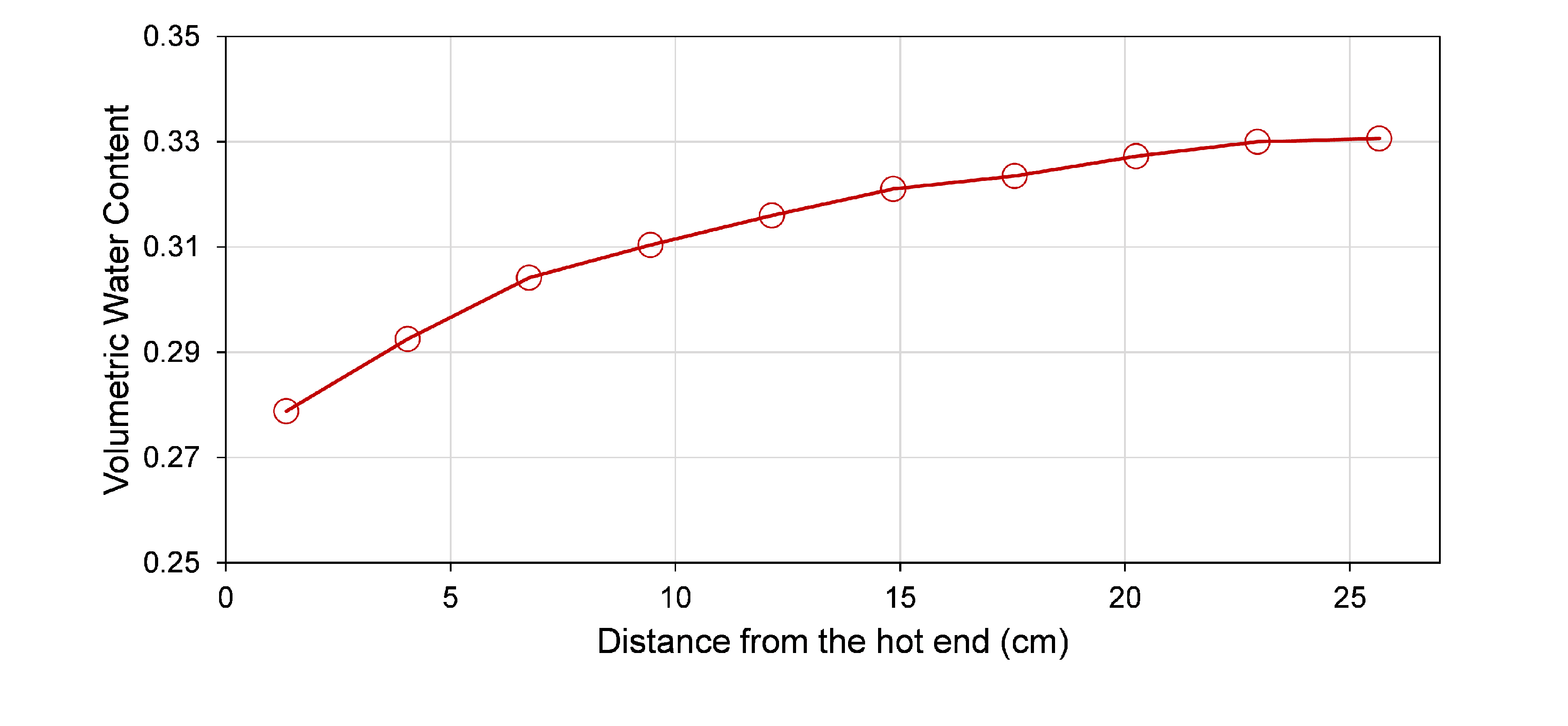
The soil has a thermal diffusivity of $1\times 10^{-7}$ , a saturated hydraulic conductivity of $3.2\times 10^{-6}$ , a residual and saturated water content of 0.05 and 0.535 respectively, a gain factor for thermally induced water flux of 5, a Young's modulus of 0.1 MPa, a Poisson's ratio of 0.3, a poroelastic expansion coefficient of 7653 Pa, and a thermal expansion coefficient of $0.8\times 10^{-6}$ . The SWCC and unsaturated water content are formulated using van Genuchten's model and the constants in the model are n=1.48, m=0.2, and l=0.5. The initial temperature and volumetric water content are 293.15 K and 0.5, respectively. The constants for the computation of the thermal diffusivity are C${}_{1}$=0.55, C${}_{2}$=0.8, C${}_{3}$=3.07, C${}_{4}$=0.13, C${}_{s}$=2$\times 10^{6} $, C${}_{w}$=4.2$\times 10^{6} $e6, and C${}_{v}$=1.2$\times 10^{3} $. The initial soil water potential head is -7 m and the initial temperature is 293.15 K. Please simulate the THM field to predict the temperature and water distributions at the end of 5 days and compare them against the following experimental results. Also, simulate the variation of the axial deformation of the cylindrical sample within the 5 days.
$\space$Results
The following figure shows the measured distributions of volumetric water content and temperature at the time of 5 days.