
Hydrodynomechanics
Introduction
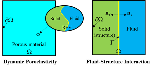
Hydrodynomechanics refers to any phenomenon involving the mechanical response of a solid and the mass and momentum transfer in a liquid. In a more general sense, the scope can be extended from liquids to fluids. In this case, hydrodynomechanics covers three application areas: dynamic poroelasticity, acoustic-structure interaction, and complete fluid-structure interaction. Dynamic poroelasticity is the hydrodynamics occurring on the level of REV. It is the dynamic extension to poromechanics. By contrast, the broad definition of the fluid-structure interaction, including the acoustic-structure interaction and the complete fluid-structure interaction, involves solid and liquid interaction on the level of regions within the computational domain. As illustrated in the following figure, the dynamic poromechanics treats the porous material as an ensemble of REVs, each of which is composed of a liquid fraction and a solid fraction. By contrast, fluid-structure interaction allows for coupling between solid and fluid regions which are at the scale of the computational domain.
Complete Fluid-Structure Interaction
The theoretical formulation consists of the equations from elastodynamics and fluid dynamics/acoustics. For the solid region, or structure, the governing mechanisms can be formulated using the Navier's equation with the inertial term:
\[\rho _{{\rm s}} \ddot{u}_{{\rm s}} =\nabla \cdot \sigma _{{\rm s}} +f_{{\rm s}} ,\]where $\sigma _{{\rm s}} $ is the stress tensor, $f_{{\rm s}} $ is the body force, $\rho _{{\rm s}} $ is the density of the solid, $u_{{\rm s}} $ the displacement vector, and $\ddot{u}_{{\rm s}} $ is the second temporal derivative of the displacement.
The governing equation for the fluid is the Navier-Stokes equations:
\[\frac{\partial \rho _{{\rm f}} }{\partial t} +\nabla \cdot \left(\rho _{{\rm f}} v_{{\rm f}} \right)=0\] \[\rho \left(\frac{\partial v_{{\rm f}} }{\partial t} +v_{{\rm f}} \cdot \nabla v_{{\rm f}} \right)=\nabla \cdot \sigma _{{\rm f}} +f_{{\rm f}} .\]The major physical mechanism to ensure the coupling of the fluid and solid regions is to satisfy the following two conditions on the boundaries between the two regions (also frequently called interface or internal boundary), $\Gamma $:
\[\dot{u}_{{\rm s}} =v_{{\rm f}} , \] and \[\sigma _{{\rm s}} \cdot n_{{\rm s}} =-\sigma _{{\rm f}} \cdot n_{{\rm f}} . \]The first equation ensures the mass conservation or no separation while the second ensures the momentum balance or mechanical equilibrium. The first condition can be replaced by the following equation when the profile of the boundary between the fluid and solid regions is smooth in both time and space,
\[u_{{\rm s}} =u_{{\rm f}} .\]According to the way to achieve the above couplings, the complete FSI techniques can be categorized into two classes: conforming mesh methods and non-conforming mesh methods. The conforming mesh methods track the location of the interface and enforce the above two equations explicitly. Gradual updates on the mesh during the solution process are usually needed as the boundary between the two regions is displaced, and therefore, the mesh within each region needs to conform with these boundary displacements. This type of method can be implemented conveniently with existing FDM, FVM, or FEM programs. A simple approach is to first enforce the non-slip boundary condition for the fluid on the fluid-solid boundary:
\[u_{{\rm f}} =0. \]On the solid side, a Neumann boundary condition can be prescribed so that the normal traction on the solid boundary is equal to the fluid pressure:
\[\sigma _{{\rm s}} \cdot n_{{\rm s}} =-\sigma _{{\rm f}} \cdot n_{{\rm f}} =-pn_{{\rm s}} ,\]where $p$ is always positive and the negative sign in front of $p$ is used to ensure that the pressure acts as a compressive stress on the solid along its boundary with the fluid.
The location of the boundary between the two regions is tracked using a moving mesh algorithm, which is available in many numerical simulation programs these days. The moving boundary is induced by the fluid pressure acting on the deformable solid structure. Therefore, the mesh displacement on the boundary between the two regions is equal to the displacement of the solid,
\[u_{{\rm mesh}} =u \space on \space\Gamma \]The movement of the mesh within the fluid and solid regions can be obtained based on the boundary movement. A common way is to use the diffusion equation, which "diffuses" the boundary displacement into the interior of each region:
\[\nabla ^{2} u_{{\rm mesh}} =0.\]On these boundaries where no boundary displacement occurs, a Neumann boundary condition can be used:
\[n\cdot \nabla u_{{\rm mesh}} =0.\]The second category is the non-conforming mesh methods, most notably, the immersed boundary method [Peskin 1977, 2002]. These methods usually enforce the velocity consistency on the boundary between the two regions instead of the displacement consistency [2012].
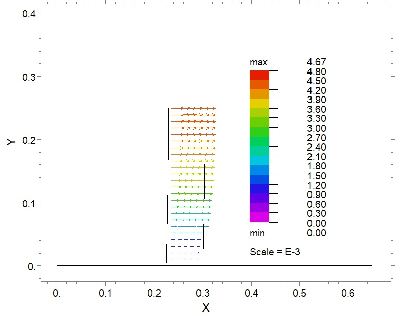
One typical example is the flow around a solid obstacle as shown in Figure 25-3. As the fluid flow encounters a structure, the structure is deformed due to the pressure exerted by the moving fluid. If the magnitude and variation of the deformations of the structure are small, the fluid flow will not be greatly affected by the resistance force from the solid.
Acoustic-Structure Interaction
In the Acoustic-Structure Interaction (ASI), we have an acoustic field in a fluid, either a liquid and a gas, and a mechanical field in a solid which is in contact with the fluid. There are two major differences between the ASI and the complete FSI. First, the N-S equations in the fluid region degenerate into a wave equation. Second, the displacement of the solid structure is generally small due to the magnitude of the disturbance while the frequency is higher than that in complete FSI. These two differences lead to the different treatments in the ASI.
The governing equation for the fluid is the mechanical wave equation. We here use the wave equation with the pressure as the dependent variable to facilitate the following formulation of coupling,
\[\nabla ^{2} p_{{\rm f}} -\frac{1}{c^{2} } \ddot{p}_{{\rm f}} =0,\] where $c$ is the wave velocity.The governing equation of the solid is still the Navier's equation with the inertial term:
\[\rho _{{\rm s}} \ddot{u}_{{\rm s}} =\nabla \cdot \sigma _{{\rm s}} +f_{{\rm s}} .\]As introduced in the previous section, the couplings for FSI requires the consistency of the displacement (or velocity) and stress on the boundary between the fluid and solid. In acoustic-structure interaction problems, the first requirement is automatically met due to the negligible solid deformation. Therefore, we just need to ensure that the stresses on two sides of the fluid-solid boundary are balanced. Mathematically, this corresponds to the following two equations:
\[n_{{\rm f}} \cdot \nabla p_{{\rm f}} =\rho \ddot{u}\] \[n_{{\rm s}} \cdot \nabla \sigma _{{\rm s}} =-pn_{{\rm f}} .\] $\space$Example
The following figure shows the cross-section of a flow channel in which water flows from the left to the right.
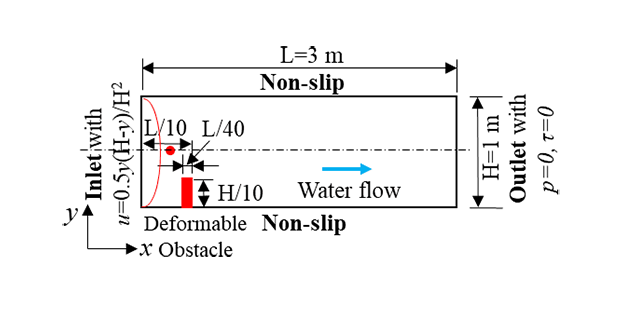
The water flow velocity on the left boundary has a profile of $0.5y(H-y)/H^2$. The right boundary has a pressure of 0 and no shear stress. The top and bottom sides are the walls of the flow channel, which can be approximated using the non-slip boundary condition. The flow channel has a length of 3 m (L) and a width (or height) of 1 m (H). An obstacle with a length of H/4 and a width of L/40 is fixed to the bottom wall at a location where the back face of the obstacle is L/10 from the left boundary. The deformation obstacle has the following mechanical properties: $\lambda $=10${}^{7}$ Pa and G=10${}^{7}$ Pa (Lamé constants). Please simulate the fluid flow and solid deformation in the process between the time when water starts moving into the channel and the time when the front of the flow passes the back face of the obstacle.